Individuals, Families and Households
The HBAI graph we discussed earlier shows the distribution of incomes of individual people, and almost all of what follows is about the welfare of individuals. But people are social beings. Most people live in households (those living alone can be thought of one-person household). Others live in other arrangements: prisons, communes, barracks, care homes and the like, but, as we’ve seen, these are typically out of scope of our datasets.
The ONS define a household as follows:
A household comprises of 1 person living alone or a group of people (not necessarily related) living at the same address who: share cooking facilities and share a living room or sitting room or dining area1
Note the need for shared facilities and shared rooms. The circumstances of the household as a whole affects the wellbeing of each individual member. There are two main issues here:
- Larger households might be more efficient than small ones. A two person household might not need twice the income of a one- person household to have the same standard of living. It’s cheaper to buy food in bulk, household might need only one fridge or cooker regardless of how large it is, and so on. Also member of larger households might be able to specialise, for example in paid or unpaid work;
- household members might not get an equal share of what’s available.
We’ll consider these in turn.
Equivalence Scales
A scale that reflects the different needs and capabilities of households of different sizes is known as an equivalence scale. If households didn’t get more efficient with size, and everyone had the same needs, then the equivalence scale would simply be 1 for a single person household, 2 for a two-person household and so on. If there are economies of scale, the numbers might be 1 for a single 1.5 for two-person, 1.8 for three. The scale might be lower for multi-person households with children, but higher for households with disabled or very elderly members.
You divide observed household income by the relevant scale to get equivalised income of the household, which is a measure of average wellbeing of the individual members. Recall that the HBAI figures we saw earlier use equivalised income2.
Where might we get such a scale? There is an equivalence scale implicit in some state benefits; for example, here are the scale rates for Job Seeker’s Allowance, a benefit paid to low-income families:
| type | £ per week | proportion of single person |
|---|---|---|
| Single Person (age 25+) | 73.10 | 1.0 |
| Couple | 114.85 | 1.57 |
| Child | 66.90 | 0.91 |
From this, you can see that if the scale for a single adult was 1.0, a 2 adult household would be 1.57, and a a two adult, one child household 2.48 (1.57+0.91).
However, these benefit amounts must themselves have come from somewhere. Can we derive and equivalence scale from first principles? One approach uses the regression techniques you learned in the previous week and the Living Costs and Food Survey I mentioned last time. The approach here dates back over 150 years, to the first ever systematic budget surveys, carried out in Germany by Ernst Engel. Engel was studying how shares of expenditure on different goods varied with income, and with family size.3 He noticed two things:
- although on average rich families spent more on food than poor ones, rich families spent a smaller share of their income on food than poor families;
- larger families had a larger share of spending on food than smaller families with the same income.
Taken together, these give us to a simple strategy to estimates equivalence scales: households of different sizes have the same well being on average when their share of spending on food is the same.
Figure XX illustrates one way of doing this, using the 2017/8 edition of the Living Costs and Food Survey (LCF) we discussed last time.
I’ve plotted total spending by each household on the x- axis against the share of food in total spending on the y- axis. Each dot represents spending by one household. I’ve grouped the LCF households into those with children (marked in orange), and those without children (in blue). The two solid lines show the average food consumption at each level of total consumption for our two classes of household - these are known as Engel Curves4. The curves are computed using the regression techniques you studied in the macroeconomics week5.
You can see that, although there is a good deal of variation, the patterns Engel observed 150 years ago are there in this dataset.
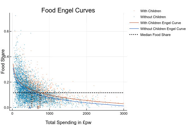
Now we can calculate an empirical equivalence scale. Pick some share of food spending - a good one might be the median food share (11.6%). That’s the dashed horizontal line. Then we look up on the Engel curves the level of total spending the two groups would on average need for this share. These are the points A and B on the diagram - for households with children, this is £747.90 (point B) and for those without, it’s £525.38 (A). The ratio between these is 1.423, which is our simple equivalence scale: our estimate is that families with children need 42% more spending than families without to enjoy the same standard of living.
A full analysis would do almost every aspect of this differently. You would want to allow for different household sizes and compositions, not just the presence or otherwise of children, and perhaps also other factors such as age, disability and the like. Nonetheless, I hope this shows you how a little bit of theory and a good dataset can be used to produce useful things in a straightforward manner. Much of the work of empirical economists, especially in the public sector, consists of doing simple exercises like this.
The HBAI data we looked at earlier is equivalised using the Modified OECD Scale6, which is as follows:
| type | proportion of single person |
|---|---|
| One Adult | 1.0 |
| Two Adults | 1.5 |
| Two Adults, 1 child | 1.8 |
| Two Adults 2 children | 2.1 |
| Two Adults 3 children | 2.4 |
and so on, with an extra 0.5 for each extra adult, and an extra 0.3 for each extra child (the OECD defines a child is someone aged 13 or under). The OECD scale is a standard scale used in many countries.7
Activity
For this activity, we invite you to explore the LCF dataset we’ve just been using.
Download our subset of the 2017/8 Living Costs and Food Survey data and its associated documentation. The dataset contains a small subset of the information on 5,376 households, including spending broken down into 13 groups and some demographic information (a few households with very extreme values have been deleted). Full details of the dataset are in the coding frame.
Mostly, these are not activities with a single right answer; instead, we invite you to explore the data using either Excel or any other tool you are familiar with. Questions 2,3 and 5 are especially difficult and you should feel under no pressure to attempt them.
- generate shares of each expenditure group in total spending (note there are two different definitions of total spending in the dataset);
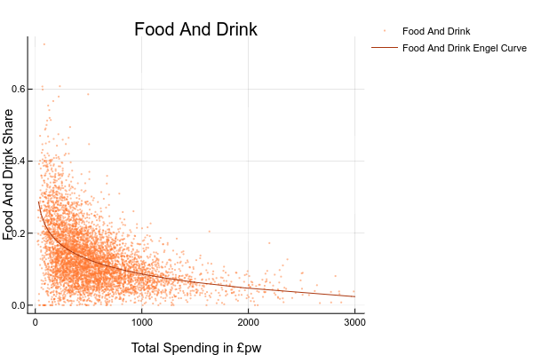
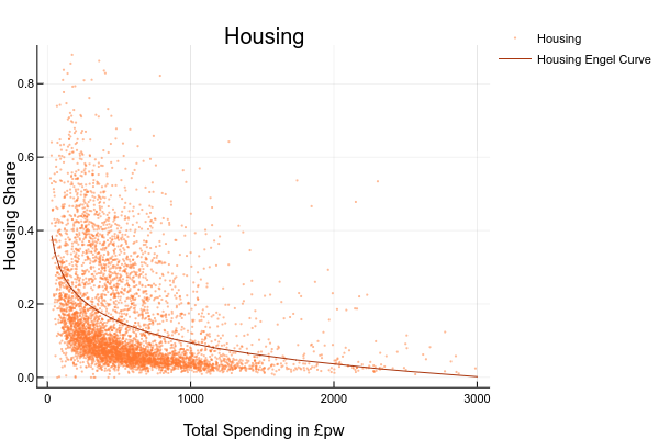
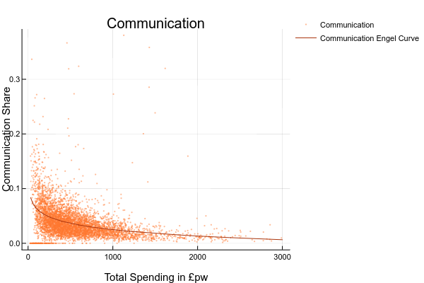
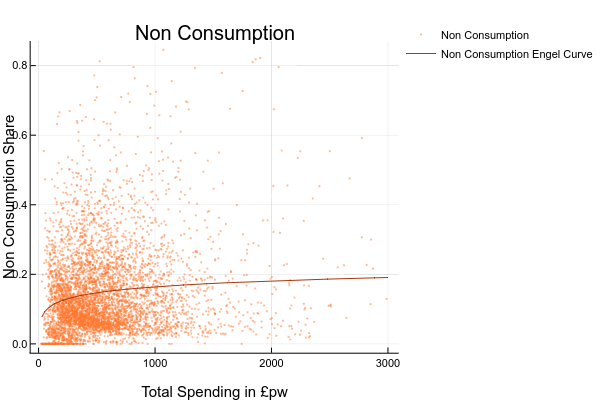
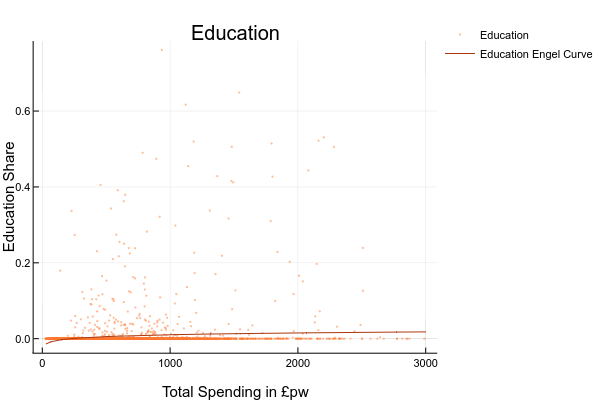
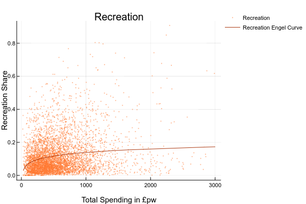
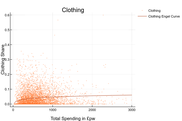
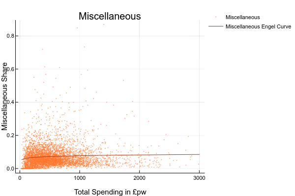
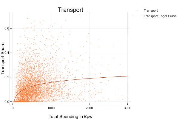
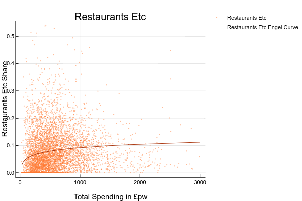
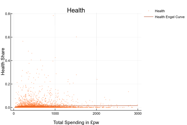
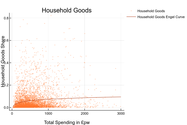
- explore the relationship between the share (or level) of spending on each good and total spending or household income. You could do this by drawing scatter plots or, if you are ambitious, estimating your own Engel curves FIXME HOW DO YOU DO RUN A REGRESSION IN EXCEL?. For this you’d need to generate a column with the logarithm of total spending ; ANSWER: The complete set of Engel Curves for this dataset is as follows:
- explore how spending on some good appears to vary for different groups. You could do this by sorting the data on economic position of the head, tenure type, or region, and then computing means and medians for subgroups;
- an alternative to Engel’s method for computing equivalence scales is Barten’s Method8, which proposes that families with and without children have the same standard of living when they have the same level of spending on adult goods.
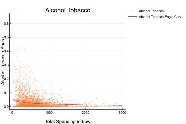
What problems do you see in applying Barten’s method to this dataset? ANSWER: a) it’s hard to define “adult goods” and it would be impossible to identify them in this dataset. The only obvious candidate is the “alcohol and tobacco” group, but there are problems with that group: we know from last time that spending on these things is under-reported, and in our data many people report not spending anything at all on these things, which makes fitting a linear relationship problematic; - A very ambitious activity might be to actually calculate rough equivalence scales using Barten’s method. You could assume the alcohol and tobacco group is representative of “adult goods”. Alternatively, try sketching out what you thing the equivalent of the Engel analysis above might look like. ANSWER: should look something like:
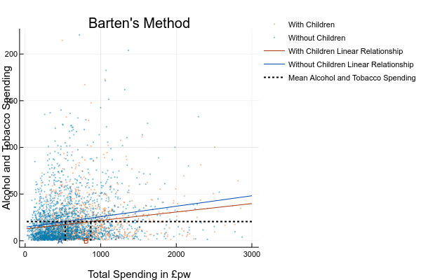 Note that here we’ve dealt with the large number of zeros simply by deleting them, estimating instead over only those households who consume these goods. Since we’re interested in the level of spending we’ve estimated a linear Engel curve. The implied equivalence scale is approximately 1.64.
End activity
Unequal distribution within households
Once we’ve equivalised our household incomes, we need to assign it to household member. Typically we just assign give everyone the average household income. But this ignores the possibility of discrimination by gender, or other characteristics such as age or disability.
Making a different assumption requires somehow looking inside households to infer how sharing of goods and the allocation of tasks actually works in practice9. In principle can use our budget surveys to examine this question, using variants of the approach above. If we can identify specifically male, female-, or children’s goods in our survey (clothing might be an example), then we can measure how spending on these vary between, for example, households where women have significant income of their own (through work or perhaps benefit payments), and households where all the income accrues to men. Alternatively, we could look at health or education outcomes - is shifting income between men and women associated with improvements in female health or school enrolment? There have been many studies, and the evidence seems mixed10. Consumption based studies tend to find no effect, whilst studies of health and education outcomes often show better outcomes in cases where incomes shifted from men to women.
Benefit Units
There’s a further subdivision of households we should briefly consider. Some state benefits such as Universal Credit or Job Seeker’s Allowance are assessed over ‘benefit units’ - roughly speaking, adults living together as a couple and any children dependent on them. A household with the a married couple and two children, and also an elderly parent, would be one household, but two benefit units, since the elderly parent would be assessed separately for means-tested benefits. In our model, and most modern analysis, benefit units are solely an indirect part of the modelling process, but in the past results were often presented at the benefit unit, rather than individual level.11
Banks, James, and Paul Johnson. Children and Household Living Standards, 1993. https://doi.org/10.1920/re.ifs.1993.0042.
Case, Anne, and Angus Deaton. Consumption, Health, Gender, and Poverty. Vol. 3020. World Bank Publications, 2003. https://rpds.princeton.edu/sites/rpds/files/media/case_deaton_consumption_health_gender.pdf.
Chai, Andreas, and Alessio Moneta. “Retrospectives: Engel Curves.” Journal of Economic Perspectives 24, no. 1 (March 2010): 225–40. https://doi.org/10.1257/jep.24.1.225.
Deaton, Angus. The Analysis of Household Surveys. Washington, DC: World Bank, 2019. https://doi.org/10.1596/978-1-4648-1331-3.
DWP. “HBAI Documentation, Appendix 2 - Methodology,” 2015. https://assets.publishing.service.gov.uk/government/uploads/system/uploads/attachment_data/file/200775/appendix_2_hbai12.pdf.
Hagenaars, A, K de Vos, and M Zaidi. Poverty Statistics in the Late 1980s: Research Based on Micro-Data. Luxembourg: Office for Official Publications of the European Communities, 1994.
Horsfield, Giles. “Living Costs and Food Survey - Methodology.” Office for National Statistics, 2016. https://cy.ons.gov.uk/peoplepopulationandcommunity/personalandhouseholdfinances/incomeandwealth/compendium/familyspending/2015/methodology#description-of-the-survey.
OECD. “WHAT ARE EQUIVALENCE SCALES?” OECD, 1995. http://www.oecd.org/eco/growth/OECD-Note-EquivalenceScales.pdf.